Compressing LLMs with Python

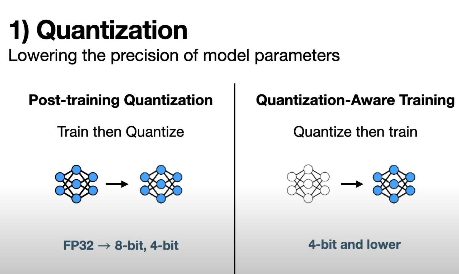
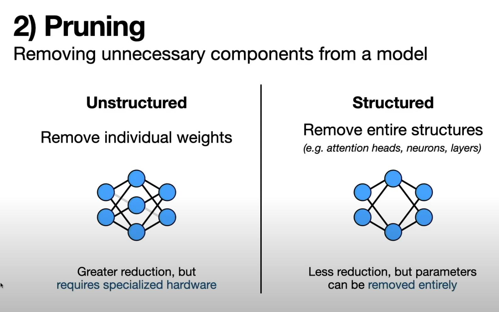
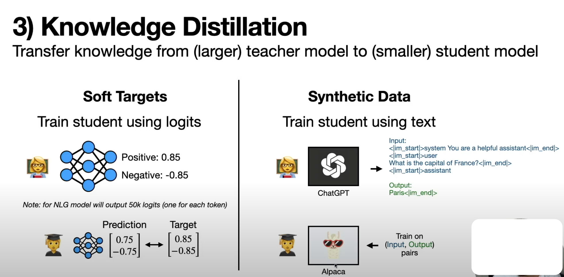
(00:00) large language models have demonstrated impressive performance across a wide range of use cases while this is largely due to their immense scale deploying these massive models to solve real world problems can be challenging in this video I’m going to discuss how we can overcome these challenges by compressing llms I’ll start with a highlevel overview of key Concepts and then dive into a specific example with python code and if you’re new here welcome I’m I make videos about data science and Entrepreneurship if you enjoy this (00:34) content please consider subscribing that’s a great no cost way you can support me in all the videos that I make last year the Mantra and AI seemed to be bigger is better where the equation for creating better models was more data plus more parameters plus more compute and we can see over time large language models just kept getting larger and larger this is a figure from reference 11 down here and we can see over time models kept getting bigger and bigger so in 2018 large meant something around 100 million parameters in 2019 with gpt2 we (01:11) were up to 1 billion parameters then came gpt3 which was around 100 billion parameters then we have more recent language models which have a trillion parameters or more there’s no doubt that this equation actually works GPT 4 is objectively better than gpt3 and everything that came before it however there’s a problem with creating bigger and bigger models simply put bigger models come with higher costs so just to put this into computational terms a 100 billion parameter model is going to take up 200 GB of storage and then if you (01:48) want to use this model you got to fit this massive thing into the memory of your machine so needless to say this comes with high compute costs so it’s probably not something that’ll run on your laptop you’re going to need a lot more compute than that it comes with higher Financial costs and then of course it comes with a higher environmental cost but what if there was a way we could make these Large Scale Models a lot smaller this is the motivation of model compression which aims to reduce the size of a machine (02:19) learning model without sacrificing its performance so if we’re able to pull this off by taking a massive model and shrinking it down to a smaller model this means we could run one of these models on our laptop or even on other devices like cell phones or SmartWatches or other types of devices not only does this Foster greater accessibility for this technology it also promotes user privacy because these models can be run on device and user information does not need to be sent to a remote server for inference this also means less Financial (02:55) cost and of course the negative environmental impact can be a lot smaller here I’m going to talk about three different ways we can compress these models the first is quantization the second is pruning and the third approach is called knowledge distillation starting with quantization although this might sound like a scary and sophisticated word it’s a very simple idea quantization consists of lowering the Precision of model parameters and you can think of this like taking a high resolution photo and converting it to a lower resolution one (03:29) that still captures the main features of the image and to put this into computational terms you might take a model whose model parameters are represented in fp32 so using 32 bits and translating the parameters into int 8 just to get a sense of this the number seven represented in fp32 looks something like this so the computer has to keep track of all these binary digits just to encode a single parameter however if that same parameter is represented in in eight that’ll look something like this it’s a fourth of the (04:03) memory footprint if you want more details on how quantization Works under the hood I talked more about it in a previous video of this series on Q Laura I’ll link that here for those who are interested when it comes to implementing quantization on large language models there are two popular categories of approaches the first is called post trining quantization and the basic idea here is you train your model and then quantize it the key upside of this is that this allows you to take models that other people have trained and then you (04:35) can take them and quantize them without any additional training or data curation using this approach you can take these off-the-shelf models that might be encoded in fp32 and convert the parameters to 8bit or even 4bit however if you want to compress Beyond 4bit post-training quantization typically leads to a degradation in model performance for situations where even more compression is needed we can turn to another set of approaches known as quantization aware training this essentially flips the order where one (05:10) quantizes the model first and then trains IT training models in lower Precision is a powerful way to get compact models that still have good performance this means parameters can be encoded with even fewer than four bits for example in reference number six the authors were able to create a one bit model that mat matched the performance of the original llama model but of course the downside of quantization aware training is that it is significantly more sophisticated than post-training quantization because one (05:41) has to train the quantized model from scratch the second compression approach is pruning which consists of removing unnecessary components from a model so an analogy here is that pruning is like clipping off dead branches from a tree it reduces the tree’s size without harming it to put this in terms of parameters we might have a 100 billion parameter model but then through pruning we might reduce it down to 60 billion parameters while there are a wide range of pruning approaches out there they can be broadly classified into two (06:14) categories the first is called unstructured pruning which consists of removing individual weights or parameters from the model showing that visually if this is our original model here unstructured pruning might consist of zeroing out the these two weights in the model the key benefit of unstructured pruning is that since it’s operating on this granular scale of individual weights it can result in a significant reduction of non-trivial model parameters however there’s a key caveat here since we’re just taking (06:47) model weights and turning them into zeros this is going to result in sparse Matrix operations to get predictions from our model in other words The Matrix multiplications involved in generating a prediction from our model will consist of a lot of zeros and this isn’t something that normal Hardware can do any faster than nonsparse Matrix operations which means that one needs specialized Hardware that’s designed to optimize these sparse Matrix operations in order to realize the benefits of unstructured pruning on the other hand (07:21) we have structured pruning which instead of removing individual weights it removes entire structures from the model this can be think things like attention heads neurons or even entire layers so visually what this might look like is if this is our original model we might remove this entire neuron from the model which does not result in the sparse Matrix operations that we see in unstructured pruning while this does result in less opportunities for model reduction it allows one to completely remove parameters from the model if you (07:56) want to explore specific unstructured and structured pruning techniques check out out reference number five which provides a nice survey of these approaches the final way we can compress an llm is via knowledge distillation this is where we transfer Knowledge from a larger model into a smaller one this is just like how we all learn at school where we have a teacher who has much more experience in a particular subject transferring their knowledge to the students in the context of large language models the teacher model might (08:28) have a 100 billion parameters which are then distilled to a student model which might have just 50 billion parameters again there are a couple of ways that we can achieve this the first is using soft targets which consists of training the student model using the logits from the teacher model what that means is let’s say we have our teacher model here and let’s say it performs sentiment analysis so given a chunk of text it’ll label that text as either positive sentiment or negative sentiment the way these model models work is that (09:00) the raw outputs are not just a positive or negative prediction but rather there’s a prediction for each class known as a logit for example let’s say the logit for the positive class is 0.85 and the logit for the negative class is minus 0.85 what this is indicating is that the input text is more likely to be positive sentiment than negative sentiment and this is exactly how text generation models like l 3. (09:32) 1 or gp4 work under the hood however instead of having two output logits these models will have tens of thousands of output lits corresponding to each token in its vocabulary these lits are then converted into probabilities and then these probabilities can be sampled to generate text one token at a time so we can actually use these loits to do knowledge distillation so the way that works is we’ll take our smaller student model have it generate predictions and then we’ll compare those predictions to the teacher model’s predictions for the same (10:07) input text and the reason these are called Soft targets is because the predictions of the student model aren’t compared to a zero or one ground truth but rather a softer fuzzier probability distribution this turns out to be an effective strategy because using all the output logits from the teacher model provides richer information to the student model to learn from another another way to achieve knowledge distillation is instead of using logits to train the student model one can use synthetic data generated by the teacher (10:39) model a popular example of this was the alpaca model which took synthetic data generated from the original chat GPT and used it to perform instruction tuning on llama 7B in other words chat GPT was used to generate these input output pairs of input prompts from users and out put responses from the model which were then used to endow this llama 7B model with the ability to follow instructions and follow user prompts so now with a basic understanding of the key Concepts behind model compression let’s see what this looks like in code (11:17) as always the example code here is freely available on the GitHub additionally all the models derived here and the data set used for training is also freely available on the hugging face Hub and we’ll be using python for this example as well as pytorch the example here is we’re going to take a text classifier and compress it using knowledge distillation and quantization so that’s one thing I actually forgot to mention is that these three different compression approaches of quantization pruning and knowledge distillation are (11:49) often independent of one another which means that we can combine multiple approaches to achieve maximum model compression so here I’m going to combine knowledge distillation with quantization to achieve a 7x reduction in model size the first step here is to do some imports many of these are hugging face libraries so data sets is from hugging face we’ll import some things from Transformers we’re going to import some things from pytorch and then finally I’m going to import some evaluation metrics (12:20) from psyit learn then I’ll import the data set with one line of code and this is something I’ve made available on the hugging face Hub it consists of a training testing and validation data set with a 70515 split so it’s 2100 examples of data in the training data set and then 450 examples in the testing and validation and the data set consists of two columns the First Column are website URLs and the second column is a binary label of whether that URL is a fishing website or not a fishing website so this (12:54) is actually a very practical use case used by email providers or cyber security folks that may want to ensure that links are safe before presenting them to end users with the data loaded in we’ll load in our teacher model here to speed things up I used the freely available GPU on Google collab so I’m importing that GPU as a device here next I’m going to load in the teacher model which is a model I ftuned on This fishing classification task we can load in the model’s tokenizer and the model itself using these two lines of code (13:28) here and then using this two method I’m loading the model onto the GPU then we can load in our student model so here we’re going to create a model from scratch I’m going to copy the architecture of distill bir to initialize the model however I’m going to drop four of the attention heads from each layer additionally I’m going to drop two of the layers from the model in other words each attention layer has 12 attention heads so I’m going to reduce that to eight and the original architecture has six layers and I’m (13:57) going to reduce that down to four then I’m going to use this distill BT for sequence classification object what that does is it’ll load in this distill BT architecture with these modifications and then slap on top of it a classification head in other words the model instead of generating text is going to perform text classification we’re also going to load the student model onto the GPU and just to get a sense of the scale here the teacher model has 109 million parameters and takes up 438 megab of memory while the (14:28) student model here here consists of 52.8 million parameters and takes up 211 MB of memory the reason I’m using relatively small models by today’s standard is that this is what I can easily run on the free GPU on collab but if you have beefier gpus or more compute at your disposal you can take this code and just plug in bigger models and it should work just fine so the data set that we loaded in consists of plain text with a label so before we can actually use the this data we’ll need to tokenize (15:01) it here I defined a simple pre-processing strategy so what’s happening here is each URL is being converted into a sequence of Tokens The Tokens are being truncated so they’re not too long and then within each batch of examples the shorter sequences are going to be padded so all the examples have the same length and this is important so we can convert it into a pytorch tensor and efficiently do the computation with the gpus this the pre-processing function the the actual transformation happens in this line of (15:31) code so we take the data set and then we map it into tokenized Data making sure that we are using batches and then we’re converting it into a pytorch format where we have columns for the tokens the attention mask and the target labels another thing we need to do is Define an evaluation function so this will allow us to compute evaluation metrics during model training and so there’s a lot happening here so I’m going to go through it line by line first we’re putting the model into eval mode instead (16:00) of training mode we’re initializing two lists one list is for model predictions another list is for labels here we’re going to disable gradient calculations then batch by batch we’re going to do the following first we’re going to load all the data onto the GPU so that’s the input tokens the attention mask and the labels then we’re going to perform the forward pass so we’re going to compute model outputs and then we’re going to extract the logits from the outputs this lits variable here will actually consist (16:28) of two numbers one one corresponding to the probability that the URL is fishing and another corresponding to the probability that the URL is not fishing so in order to turn this into a binary classification in other words the URL is fishing or is not fishing we can take the ARG Max of this logits variable and then that’ll be our prediction and then we can append the predictions and the ground truth label to these lists we initialized earlier once we do that for all the batches we can compute the accuracy precision recall and F1 score (17:00) for all the data in one go next we’re going to define a custom loss function and the way we’re going to do that is we’re going to use both soft Targets in other words the logits from the teacher model and the ground truth labels and so the way we’re doing that here is we’re going to compute a distillation loss as well as a hard loss and then we’re going to combine those into a final loss so to get the distillation loss we’ll first compute the soft targets so these are the teachers logits and then we’re going (17:29) to convert those logits into probabilities in order to generate probabilities from the teacher models logits we can use the soft Max function and it’s common practice to divide the teacher logits by a temperature parameter which will increase the entropy of the probability distribution so we generate a probability distribution corresponding to the teacher’s prediction and then a probability distribution corresponding to the students prediction and now that we have two probability distributions one from the teacher model one from the (18:01) student model we can compare their differences using the KL Divergence pytorch has a built-in method that does that so we can just easily compute the difference between these two probability distributions using this line of code here and then we can compute the hard loss so instead of comparing the student model’s predictions to the teacher model’s predictions we’re going to compare them to the ground truth label and then we’ll use the cross entropy loss to compare those probabilities distributions and then finally we can (18:31) combine these losses by adding them together and adding this Alpha parameter which controls how much weight we’re giving to the distillation loss versus the hard loss next we’ll Define the hyperparameter so here I use a badge size of 32 put the learning rate as . (18:51) 001 we’ll do five Epoch we’ll set the temperature that we use in our loss function at two and then we’ll set the alpha so the relative weights of the distillation loss versus the hard loss as 0.5 so we’ll give equal weight to both types of losses then we’ll Define our Optimizer so we’ll use atom then we’ll create two data loaders we’ll have a data loader to control the flow of batches for the training data as well as the testing data then we’ll train the model using pytorch so we put the student model into train mode and then (19:21) train it we have two for Loops here so we have one for the epoch one for the batches and it’s a similar thing as to what we saw in the evaluation function so we’ll load each batch onto the GPU we’ll compute the outputs of the teacher model and then since we’re not training the teacher model there’s no need to calculate gradients so we can avoid that using this syntax here then we’ll pass through the student model to generate its outputs and extract its logits we’ll compute the loss value using our (19:47) distillation loss that we defined earlier and then we’ll perform the back propagation sorry the script was too long so I have to extend it like this but once we make it through every single batch we can print the performance metric tricks after each Epoch so we’ll print the accuracy precision recall F1 score for the teacher model and then the accuracy precision recall F1 score for the student model and then we’ll be sure to put the student model back into train mode because this evaluate model function that we defined earlier puts it (20:16) into eval mode so I know this was a ton of code maybe way more code than you were hoping to get into but here are the results of the training so we have five Epoch here and we can see the loss is going down which is a good sign so it bumped up in Epoch 4 but then it dropped back down in Epoch 5 which is very normal and then we can compare the performance of the teacher and student models so of course since we’re not updating the teacher model its accuracy is going to stay the same across all Epoch cuz it’s not changing but we can (20:46) see the student model performance get better and better across each Epoch and then once we get to Epoch number five the student model is actually performing better than the teacher across all evaluation metrics next we can evaluate the performance of the teacher and student models using the independent validation data set so the training set is used to update model parameters the testing data set is used in tuning the hyperparameters of the model and the validation set wasn’t touched so this will give us a fair evaluation of each (21:18) model and for that we again see that the student model is performing better than the teacher model across all evaluation metrics this is one of the other upsides of model compression if your base model if your teacher model is overparameterized meaning that it has way too many internal parameters relative to the task that it’s trying to achieve actually compressing the model not only reduces the memory footprint but also it can lead to better performance because it’s removing a lot of the noisy and redundant structures (21:51) within the model but we can go one step further so we did knowledge distillation let’s see how we can quantize this model first I’ll push the student model to the hugging face Hub and then we’ll load it back in using the bits and bytes integration in the Transformers Library so we’ll use the bits and bytes config so we’ll load it in for bit we’ll use the normal float data type described in the Cur paper and all this is is a clever way of doing the quantization to take advantage that model parameters (22:21) tend to be normally distributed so you can be a bit more clever in how you quantize the values and I talk more about that in the Cur video that I mentioned earlier next we’ll set the compute data type as brain float 16 and then finally we’ll do double quantization which is another thing described in the Cur paper once we set up this config we can simply just load in our student model from the hugging face hub using this config file so the result of that is we have still the same number of parameters 52.8 million but (22:54) we’ve reduced the memory footprint so we went from 21 megab down to 62.7 megab then comparing that to our original teacher model we started with we cut the number of model parameters in half and then we reduced the memory footprint by about 7x but we’re not done yet so just cuz we reduced the model size that doesn’t mean that we still maintain the performance so now let’s evaluate the performance of the quantize model here we see we actually get another performance game post quantization so intuitively we can understand this (23:25) through the aam’s razor principle which says that simpler models are better so this might be indicating that there’s even more opportunity in knowledge distillation for this specific task all right so that brings us to the end if you enjoyed this video and you want to learn more check out the blog in towards data science and although this is a member only story like all my other videos you can access it completely for free using the friend Link in the description below additionally if you enjoyed this video you may enjoy the (23:55) other videos in my llm series and you can check those out by clicking on on the playlist linked here and as always thank you so much for your time and thanks for watching

Image List